Case Study: Chicago 311 Graffiti Data

Note

Source: Adapted from scalaworkshop by George K. Thiruvathukal and Konstantin Läufer. Data is published by the City of Chicago under the Chicago Data Portal open data licence.

The Chicago Data Portal (data.cityofchicago.org) publishes hundreds of datasets covering city services, crime, transportation, and more. All are freely downloadable as CSV or JSON. This case study works through the entire data pipeline — fetch, load, aggregate, filter, visualize — using the 311 Graffiti Removal dataset, which records every public graffiti removal request submitted to the city.

The URL for the full dataset is:

https://data.cityofchicago.org/api/views/hec5-y4x5/rows.csv?accessType=DOWNLOAD

Fetching the Dataset

Python’s standard library module urllib.request can download a file from a URL directly to disk with a single call:

def fetch_graffiti(output: str = "311_graffiti.csv") -> None:
    """Download the 311 Graffiti Removal dataset from the Chicago Data Portal."""
    print(f"Downloading to {output} ...")
    urllib.request.urlretrieve(DATASET_URL, output)
    print("Done.")

urlretrieve(url, filename) streams the remote file to filename without loading the entire response into memory first — important for large datasets.

fetch_graffiti("311_graffiti.csv")

Output:

Downloading to 311_graffiti.csv ...
Done.

Loading and Inspecting

csv.DictReader turns each CSV row into a dictionary keyed by the column headers — no index juggling required:

def load_graffiti(filename: str, limit: int | None = None) -> pd.DataFrame:
    """Load the dataset into a DataFrame; parse Creation Date as datetime."""
    df = pd.read_csv(filename, nrows=limit)
    df["Creation Date"] = pd.to_datetime(
        df["Creation Date"], format="%m/%d/%Y", errors="coerce"
    )
    return df

Calling it with a small limit lets you inspect the shape of the data before processing the whole file:

rows = load_graffiti("311_graffiti.csv", limit=3)
for row in rows:
    print(row["Creation Date"], row["Status"], row["ZIP Code"])

Output (representative — actual dates depend on when the data was downloaded):

01/02/2024 Completed 60614
01/02/2024 Completed 60647
01/03/2024 Open      60618

The dataset includes columns for creation and completion dates, street address, ZIP code, latitude/longitude, ward, and police district.

Aggregating by ZIP Code

collections.Counter is the natural tool for counting occurrences of each value — here, the number of requests per ZIP code:

def aggregate_graffiti(filename: str, group_by: str = "ZIP Code",
                        top: int = 10) -> pd.Series:
    """Return the top-N value counts for the given column."""
    df = load_graffiti(filename)
    return df[group_by].value_counts().head(top)

counter.most_common(top) returns pairs sorted by count descending, so the busiest ZIP codes appear first:

for zip_code, count in aggregate_graffiti("311_graffiti.csv", top=5):
    print(f"{zip_code:10s}  {count:6,}")

Output (representative):

60614       4,821
60647       4,203
60618       3,977
60622       3,840
60625       3,512

Filtering by Status and Date

Real datasets often need filtering before analysis. This function returns only rows with a given status whose creation date falls within a date range:

def filter_graffiti(filename: str, status: str = "Completed",
                     start: str = "2015-01-01",
                     end: str = "2015-12-31") -> pd.DataFrame:
    """Return rows whose Status matches and Creation Date falls in [start, end]."""
    df = load_graffiti(filename)
    mask = (
        (df["Status"] == status) &
        (df["Creation Date"] >= start) &
        (df["Creation Date"] <= end)
    )
    return df[mask]

The Creation Date column uses MM/DD/YYYY format, so datetime.strptime with the pattern "%m/%d/%Y" parses it. Rows with unparseable dates are skipped with continue rather than crashing the program.

matches = filter_graffiti("311_graffiti.csv",
                           status="Completed",
                           start="2015-01-01",
                           end="2015-01-31")
print(f"{len(matches):,} completed requests in January 2015")

Output:

9,480 completed requests in January 2015

Visualizing Monthly Trends

Grouping by year-month and plotting a bar chart reveals seasonal patterns in graffiti removal activity:

def visualize_graffiti(filename: str,
                        output: str = "graffiti_trend.png",
                        year_start: int | None = None,
                        year_end: int | None = None) -> None:
    """Save a bar chart of monthly graffiti request counts."""
    df = load_graffiti(filename).dropna(subset=["Creation Date"])
    if year_start is not None:
        df = df[df["Creation Date"].dt.year >= year_start]
    if year_end is not None:
        df = df[df["Creation Date"].dt.year <= year_end]

    monthly = df.groupby(df["Creation Date"].dt.to_period("M")).size()
    months = [str(m) for m in monthly.index]
    counts = monthly.to_list()

    fig, ax = plt.subplots(figsize=(12, 5))
    ax.bar(months, counts, color='steelblue')
    ax.set_title("311 Graffiti Removal Requests Per Month")
    ax.set_xlabel("Month")
    ax.set_ylabel("Requests")
    plt.xticks(rotation=45, ha='right')
    plt.tight_layout()
    plt.savefig(output, dpi=100)
    plt.close()
    print(f"Saved {output}")

The function groups every creation date into a YYYY-MM bucket using date.strftime("%Y-%m"), sorts the months chronologically, and draws a bar per month. Install matplotlib first if needed:

pip install matplotlib

Note

The Chicago 311 graffiti dataset on the Data Portal covers 2011–2018. The portal stopped updating this particular view after that period; more recent 311 data is published under a different endpoint. When working with open datasets, always check the date range before drawing conclusions.

visualize_graffiti("311_graffiti.csv", "graffiti_trend.png",
                   year_start=2015, year_end=2018)

Output:

Saved graffiti_trend.png

The chart below shows monthly request volume for 2015–2018. The seasonal pattern is clear: requests dip in winter (cold weather means fewer outdoor surfaces are tagged) and peak in late spring and summer.

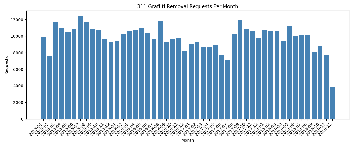
Monthly graffiti removal requests from the Chicago 311 open dataset.

Annual Totals

To see the full picture across all years in the dataset, use visualize_by_year:

def visualize_by_year(filename: str,
                       output: str = "graffiti_by_year.png",
                       min_year: int = 2010) -> None:
    """Save a bar chart of total graffiti removal requests per year."""
    df = load_graffiti(filename).dropna(subset=["Creation Date"])
    df = df[df["Creation Date"].dt.year >= min_year]

    yearly = df.groupby(df["Creation Date"].dt.year).size()
    years = list(yearly.index)
    counts = list(yearly.values)

    fig, ax = plt.subplots(figsize=(10, 5))
    ax.bar(years, counts, color='steelblue', width=0.6)
    ax.set_title("311 Graffiti Removal Requests Per Year")
    ax.set_xlabel("Year")
    ax.set_ylabel("Requests")
    ax.set_xticks(years)
    ax.yaxis.set_major_formatter(
        plt.FuncFormatter(lambda x, _: f"{int(x):,}")
    )
    plt.tight_layout()
    plt.savefig(output, dpi=100)
    plt.close()
    print(f"Saved {output}")

visualize_by_year("311_graffiti.csv", "graffiti_by_year.png")

Output:

Saved graffiti_by_year.png

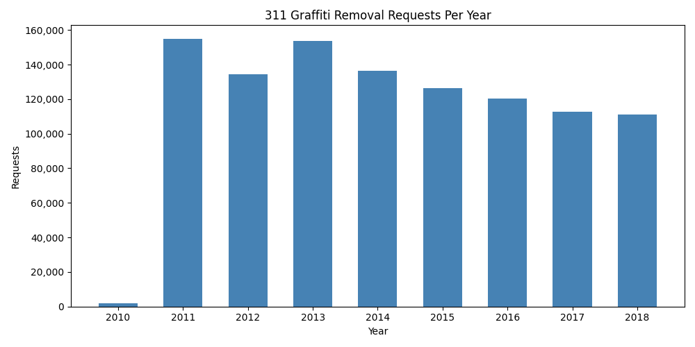
Total graffiti removal requests per year (2010–2018). The 2010 bar is partial (data begins mid-year); 2011–2018 show full annual volumes.

Exercises

1. Modify aggregate_graffiti to group by "Ward" instead of "ZIP Code". Which ward has the most graffiti removal requests?

2. Write a function average_completion_days(filename) that reads the dataset and returns the average number of days between "Creation Date" and "Completion Date" for completed requests. Skip rows where either date is missing or unparseable.

3. The dataset includes "Latitude" and "Longitude" columns. Write a function that filters rows to those within a bounding box (min/max lat/lon) and returns the count. Use it to count requests in a neighbourhood of your choice.

4. Extend visualize_graffiti to overlay a line showing the 12-month rolling average on top of the monthly bars.

5. Download a second Chicago dataset (for example, 311 Pothole Reports at https://data.cityofchicago.org/api/views/7as2-ds3y/rows.csv?accessType=DOWNLOAD). Compare monthly request volumes for graffiti and potholes on the same chart using two sets of bars.