Data Analysis with Pandas#
Note
Source: Adapted from COMP 180 course notebooks developed by George K. Thiruvathukal, Daniel Henriques Moreira, and Mohammed Abuhamad. Rewritten for this book as regular Python examples and Sphinx code blocks rather than Jupyter notebooks.
Many useful programs work with tabular data: rows and columns of
related values. A spreadsheet is tabular data. So is a CSV file, a
database query result, and many web API responses. Earlier chapters
showed how to represent records with dictionaries and collections of
records with lists of dictionaries. The
pandas library builds on those ideas and gives you a higher-level
object, the DataFrame, for working with whole tables at once.
This chapter introduces just enough pandas to make the later data case
studies easier to read. You will create a DataFrame, select rows and
columns, sort and filter data, group rows, compute summary statistics,
and make a first chart with matplotlib.
Install pandas and matplotlib if needed:
pip install pandas matplotlib
Creating a DataFrame#
A DataFrame can be built from a list of dictionaries. Each dictionary describes one row. The dictionary keys become column names:
COUNTRIES = [
    {
        "Country": "Canada",
        "Continent": "North America",
        "Population": 38.8,
        "GDP": 2140,
        "Area": 9_984_670,
        "HDI": 0.936,
    },
    {
        "Country": "France",
        "Continent": "Europe",
        "Population": 68.0,
        "GDP": 3030,
        "Area": 551_695,
        "HDI": 0.910,
    },
    {
        "Country": "Germany",
        "Continent": "Europe",
        "Population": 84.4,
        "GDP": 4450,
        "Area": 357_114,
        "HDI": 0.950,
    },
    {
        "Country": "Italy",
        "Continent": "Europe",
        "Population": 58.9,
        "GDP": 2300,
        "Area": 301_340,
        "HDI": 0.906,
    },
    {
        "Country": "Japan",
        "Continent": "Asia",
        "Population": 124.5,
        "GDP": 4210,
        "Area": 377_975,
        "HDI": 0.925,
    },
    {
        "Country": "United Kingdom",
        "Continent": "Europe",
        "Population": 67.7,
        "GDP": 3340,
        "Area": 243_610,
        "HDI": 0.940,
    },
    {
        "Country": "United States",
        "Continent": "North America",
        "Population": 334.9,
        "GDP": 27360,
        "Area": 9_833_517,
        "HDI": 0.927,
    },
]
The following function converts that list into a DataFrame and uses the
"Country" column as the row index:
def create_country_dataframe() -> pd.DataFrame:
    """Return a DataFrame indexed by country name."""
    df = pd.DataFrame(COUNTRIES)
    return df.set_index("Country")
The index is the label pandas uses for each row. A meaningful index lets you ask for rows by name instead of by position.
countries = create_country_dataframe()
print(countries)
Output:
                      Continent  Population    GDP     Area    HDI
Country
Canada            North America        38.8   2140  9984670  0.936
France                   Europe        68.0   3030   551695  0.910
Germany                  Europe        84.4   4450   357114  0.950
Italy                    Europe        58.9   2300   301340  0.906
Japan                      Asia       124.5   4210   377975  0.925
United Kingdom           Europe        67.7   3340   243610  0.940
United States     North America       334.9  27360  9833517  0.927
Summary Statistics#
describe gives a quick numerical summary of every numeric column:
print(countries.describe())
Output:
       Population           GDP          Area       HDI
count    7.000000      7.000000  7.000000e+00  7.000000
mean   111.028571   6690.000000  3.092846e+06  0.927714
std    102.202539   9156.141837  4.657552e+06  0.015861
min     38.800000   2140.000000  2.436100e+05  0.906000
25%     63.300000   2665.000000  3.292270e+05  0.917500
50%     68.000000   3340.000000  3.779750e+05  0.927000
75%    104.450000   4330.000000  5.192606e+06  0.938000
max    334.900000  27360.000000  9.984670e+06  0.950000
This is often the first thing to do after loading unfamiliar data. It shows the count, average, spread, and range of the numeric columns. It can also reveal suspicious values: a population of zero, a negative area, or a missing column that did not load as a number.
Selecting Rows and Columns#
There are three common selection patterns.
Use square brackets with column names to select columns:
print(countries[["Population", "GDP"]])
Output:
                Population    GDP
Country
Canada                38.8   2140
France                68.0   3030
Germany               84.4   4450
Italy                 58.9   2300
Japan                124.5   4210
United Kingdom        67.7   3340
United States        334.9  27360
Use loc to select by row and column labels:
print(countries.loc[["France", "Japan"], ["Population", "GDP"]])
Output:
         Population   GDP
Country
France         68.0  3030
Japan         124.5  4210
Use iloc to select by integer position:
print(countries.iloc[0:3])
Output:
                 Continent  Population   GDP     Area    HDI
Country
Canada       North America        38.8  2140  9984670  0.936
France              Europe        68.0  3030   551695  0.910
Germany             Europe        84.4  4450   357114  0.950
The distinction matters. loc uses names from the DataFrame’s
index and columns. iloc uses zero-based positions, like list
indexing.
Filtering and Sorting#
Filtering keeps only rows that satisfy a condition. This expression keeps countries whose population is at least 60 million:
large = countries[countries["Population"] >= 60]
print(large.sort_values("Population", ascending=False))
Output:
                      Continent  Population    GDP     Area    HDI
Country
United States     North America       334.9  27360  9833517  0.927
Japan                      Asia       124.5   4210   377975  0.925
Germany                  Europe        84.4   4450   357114  0.950
France                   Europe        68.0   3030   551695  0.910
United Kingdom           Europe        67.7   3340   243610  0.940
The expression countries["Population"] >= 60 produces a column of
True and False values. Passing that column back into
countries[...] keeps the rows where the value is True. This is
called boolean indexing.
Grouping Rows#
Grouping collects rows that share a value, then computes something for each group. Here we group countries by continent and compute the mean population and GDP:
def summarize_countries(df: pd.DataFrame) -> pd.DataFrame:
    """Filter, sort, and group country data."""
    large = df[df["Population"] >= 60]
    print(large.sort_values("Population", ascending=False))
    print()

    by_continent = df.groupby("Continent")[["Population", "GDP"]].mean()
    return by_continent.sort_values("Population", ascending=False)
summary = summarize_countries(countries)
print(summary)
Output:
               Population      GDP
Continent
North America      186.85  14750.0
Asia               124.50   4210.0
Europe              69.75   3280.0
The expression df.groupby("Continent")[["Population", "GDP"]].mean()
means: split the rows by continent, keep the population and GDP
columns, and compute the mean for each group.
Plotting a Bar Chart#
Tables are precise, but charts make patterns easier to see. The
matplotlib library is commonly used with pandas for plotting:
def plot_gdp(df: pd.DataFrame, output: str = "country_gdp.png") -> None:
    """Save a bar chart of GDP by country."""
    ordered = df.sort_values("GDP", ascending=False)

    fig, ax = plt.subplots(figsize=(10, 5))
    ax.bar(ordered.index, ordered["GDP"], color="steelblue")
    ax.set_title("GDP by Country")
    ax.set_xlabel("Country")
    ax.set_ylabel("GDP, billions of US dollars")
    ax.tick_params(axis="x", labelrotation=30)
    plt.tight_layout()
    plt.savefig(output, dpi=120)
    plt.close()
    print(f"Saved {output}")
plot_gdp(countries, "country_gdp.png")
Output:
Saved country_gdp.png
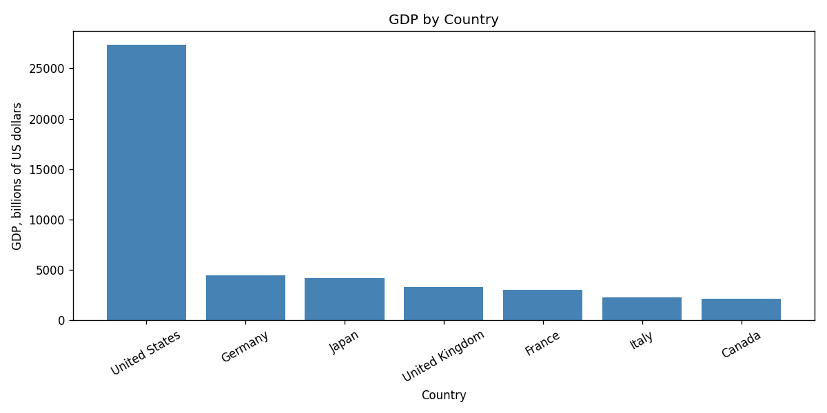
GDP by country for the sample DataFrame.#
The chart code follows the same structure you will see in later case studies: create a figure and axes, draw the chart, label the axes, tighten the layout, save the image, and close the figure.
Reading Data from CSV#
Most real data will come from a file rather than a list written inside
your program. The read_csv function loads a CSV file directly into
a DataFrame:
countries = pd.read_csv("countries.csv")
countries = countries.set_index("Country")
Once the data is loaded, the same operations apply: describe,
column selection, loc, iloc, filtering, grouping, and plotting.
That consistency is why pandas is useful. You can learn a small set of
operations and apply them to many different datasets.
Exercises#
Add a
Life Expectancycolumn to the country data. Usedescribeto summarize it.Write an expression that selects only countries in Europe.
Sort the DataFrame by
HDIfrom highest to lowest.Group by
Continentand compute the maximumHDIin each group.Modify
plot_gdpto plot population instead of GDP.