Case Study: Monte Carlo Simulation#
Note
Source: Adapted from scalaworkshop by George K. Thiruvathukal and Konstantin Läufer. Original Scala implementation at introds-scala-examples/montecarlo-scala.
Problem. How do you estimate the value of π without using any formula? One answer: throw darts randomly at a square and count how many land inside the inscribed circle.
This is a Monte Carlo simulation — a technique that uses random sampling to estimate a result that would be hard or impossible to compute analytically. The method generalises to integration, risk analysis, physics, and many other domains.
The Setup#
Draw a 2×2 square centred at the origin and inscribe a unit circle (radius 1) inside it.
Area of square  = 4
Area of circle  = π

P(random point lands inside circle) = π / 4

Therefore: π ≈ 4 × (points inside) / (total points)
The more points you throw, the closer the estimate converges to the true value.
Step 1 — Generate the Darts#
Each dart is a random point (x, y) with x and y each drawn uniformly from [-1, 1]. A dart is inside the circle when x² + y² ≤ 1:
def generate_darts(n: int) -> pd.DataFrame:
    """Generate n random darts thrown at the 2×2 square [−1,1]×[−1,1]."""
    x = [random.uniform(-1, 1) for _ in range(n)]
    y = [random.uniform(-1, 1) for _ in range(n)]
    inside = [xi * xi + yi * yi <= 1.0 for xi, yi in zip(x, y)]
    return pd.DataFrame({'x': x, 'y': y, 'inside': inside})
The function returns a DataFrame with columns x, y, and
inside, so the data is self-describing and can be saved or
analysed with standard pandas operations.
Step 2 — Save the Darts to a File#
DataFrame.to_csv writes the DataFrame to disk in one call.
Passing index=False omits the row numbers that pandas adds by
default, keeping the file clean and portable:
def save_darts(darts: pd.DataFrame, filename: str = 'darts.csv') -> None:
    """Save dart throws to a CSV file with columns x, y, inside."""
    darts.to_csv(filename, index=False)
darts = generate_darts(100_000)
save_darts(darts, "darts.csv")
Output:
$ head -3 darts.csv
x,y,inside
0.327450182,-0.645223491,True
-0.812774563,0.203948217,True
Separating generation from analysis is a deliberate design choice. Once the darts are on disk you can share the file, re-run the analysis without re-generating, or load the same dataset in a completely different script.
Step 3 — Load the Darts from a File#
pd.read_csv reconstructs the DataFrame from the saved file.
Because the inside column was written as True/False,
pandas reads it back as a boolean column automatically:
def load_darts(filename: str) -> pd.DataFrame:
    """Load a previously saved darts CSV back into a DataFrame."""
    return pd.read_csv(filename)
darts = load_darts("darts.csv")
print(darts.shape, darts.dtypes)
Output:
(100000, 3)
x        float64
y        float64
inside      bool
dtype: object
Step 4 — Estimate π#
estimate_pi works identically whether the DataFrame came from
generate_darts or load_darts — both produce the same shape
and column types. Because darts["inside"] is a boolean Series,
.sum() counts the True values directly:
def estimate_pi(darts: pd.DataFrame) -> float:
    """Estimate pi from dart throws: 4 × (inside / total)."""
    return 4.0 * darts["inside"].sum() / len(darts)
With 100 000 darts:
import math
darts = load_darts("darts.csv")
print(f"π ≈ {estimate_pi(darts):.6f}  (true: {math.pi:.6f})")
Output:
π ≈ 3.141440 (true: 3.141593)
Step 5 — Measure Convergence#
How many darts do you need? The error shrinks roughly as 1/√n — each tenfold increase in darts buys roughly one more correct decimal place at the cost of ten times the work:
def convergence_table(sizes: list[int]) -> None:
    """Print how the pi estimate improves as n grows."""
    print(f"{'n':>10}  {'π estimate':>12}  {'error':>10}")
    print("-" * 38)
    for n in sizes:
        darts = generate_darts(n)
        estimate = estimate_pi(darts)
        print(f"{n:>10,}  {estimate:>12.6f}  {abs(estimate - math.pi):>10.6f}")
convergence_table([100, 1_000, 10_000, 100_000, 1_000_000])
Output (varies due to randomness — representative run):
         n    π estimate       error
--------------------------------------
       100      3.120000    0.021593
     1,000      3.144000    0.002407
    10,000      3.138800    0.002793
   100,000      3.141440    0.000153
 1,000,000      3.141612    0.000019
Step 6 — Visualize#
A scatter plot makes the geometry tangible: blue dots inside the circle, red dots in the corners.
def plot_darts(darts: pd.DataFrame, filename: str = 'darts.png') -> None:
    """Scatter-plot dart throws, coloring inside/outside the circle differently."""
    inside  = darts[darts["inside"]]
    outside = darts[~darts["inside"]]

    fig, ax = plt.subplots(figsize=(6, 6))
    ax.scatter(inside["x"],  inside["y"],  s=0.5, color='steelblue', alpha=0.4, label='inside')
    ax.scatter(outside["x"], outside["y"], s=0.5, color='salmon',    alpha=0.4, label='outside')

    theta = [math.tau * i / 1000 for i in range(1001)]
    ax.plot([math.cos(t) for t in theta], [math.sin(t) for t in theta],
            'k-', linewidth=1.5)

    pi_est = estimate_pi(darts)
    ax.set_aspect('equal')
    ax.set_title(f'Monte Carlo: π ≈ {pi_est:.5f}  (n = {len(darts):,})')
    ax.legend(markerscale=8, loc='lower right')
    plt.tight_layout()
    plt.savefig(filename, dpi=100)
    plt.close()
    print(f"Saved {filename}")
from monte_carlo import generate_darts
darts = generate_darts(20_000)
plot_darts(darts, 'darts.png')
Install matplotlib first if needed:
pip install matplotlib
Convergence at a Glance#
The grid below shows how the estimate and the scatter of darts change as n grows across three orders of magnitude. Each panel title shows the dart count, the estimated value of π, and the time taken to generate that panel.
For large n, generating all darts at once would require tens of gigabytes
of memory. Instead, numpy is used to generate and count darts in
chunks, keeping peak memory around 160 MB regardless of n:
def _sample_and_estimate(n: int, max_display: int,
                          chunk_size: int = 10_000_000) -> tuple[float, pd.DataFrame]:
    """Return (pi_estimate, display_sample) for n darts.

    Processes in chunks of chunk_size so arbitrarily large n never requires
    more than ~160 MB of working memory (two float64 arrays of chunk_size).
    The display sample is taken from the first chunk.
    """
    import numpy as np

    inside_total = 0
    sample_x: list[float] = []
    sample_y: list[float] = []
    sample_inside: list[bool] = []
    remaining = n

    while remaining > 0:
        chunk = min(chunk_size, remaining)
        x = np.random.uniform(-1.0, 1.0, chunk)
        y = np.random.uniform(-1.0, 1.0, chunk)
        mask = x * x + y * y <= 1.0
        inside_total += int(mask.sum())

        if len(sample_x) < max_display:
            k = min(chunk, max_display - len(sample_x))
            sample_x.extend(x[:k].tolist())
            sample_y.extend(y[:k].tolist())
            sample_inside.extend(mask[:k].tolist())

        remaining -= chunk

    sample = pd.DataFrame({'x': sample_x, 'y': sample_y, 'inside': sample_inside})
    return 4.0 * inside_total / n, sample
plot_convergence_grid calls this for each panel, then plots the
display sample:
def plot_convergence_grid(sizes: list[int],
                           filename: str = 'convergence_grid.png',
                           max_display: int = 50_000) -> None:
    """Grid of scatter plots showing dart throws at multiple scales.

    The layout is determined automatically from the number of sizes.
    Pi is estimated from all n darts; only max_display points are plotted
    per panel so large n renders quickly.
    """
    if len(sizes) <= 3:
        cols, rows = len(sizes), 1
    else:
        cols = math.ceil(math.sqrt(len(sizes)))
        rows = math.ceil(len(sizes) / cols)
    theta = [math.tau * i / 1000 for i in range(1001)]
    cos_t = [math.cos(t) for t in theta]
    sin_t = [math.sin(t) for t in theta]

    fig, axes = plt.subplots(rows, cols, figsize=(5 * cols, 5 * rows))
    ax_list = list(axes.flat)

    for ax, n in zip(ax_list, sizes):
        print(f"  generating n={n:,} ...", flush=True)
        t0 = time.perf_counter()
        pi_est, sample = _sample_and_estimate(n, max_display)
        elapsed = time.perf_counter() - t0

        inside  = sample[sample["inside"]]
        outside = sample[~sample["inside"]]

        pt_size = max(0.3, 10 / (math.log10(n) ** 1.5))
        alpha   = max(0.15, 0.7 - 0.1 * math.log10(n))

        ax.scatter(inside["x"],  inside["y"],  s=pt_size, color='steelblue', alpha=alpha)
        ax.scatter(outside["x"], outside["y"], s=pt_size, color='salmon',    alpha=alpha)
        ax.plot(cos_t, sin_t, 'k-', linewidth=1.0)
        ax.set_aspect('equal')
        ax.set_xlim(-1.05, 1.05)
        ax.set_ylim(-1.05, 1.05)
        ax.set_title(f'n = {n:,}   π ≈ {pi_est:.5f}   t = {elapsed:.2f}s', fontsize=12)
        ax.set_xticks([])
        ax.set_yticks([])

    for ax in ax_list[len(sizes):]:
        ax.set_visible(False)

    fig.suptitle('Monte Carlo Estimation of π', fontsize=14)
    plt.tight_layout()
    plt.savefig(filename, dpi=100)
    plt.close()
    print(f"Saved {filename}")
plot_convergence_grid([1_000, 1_000_000, 1_000_000_000],
                       'convergence_grid.png')
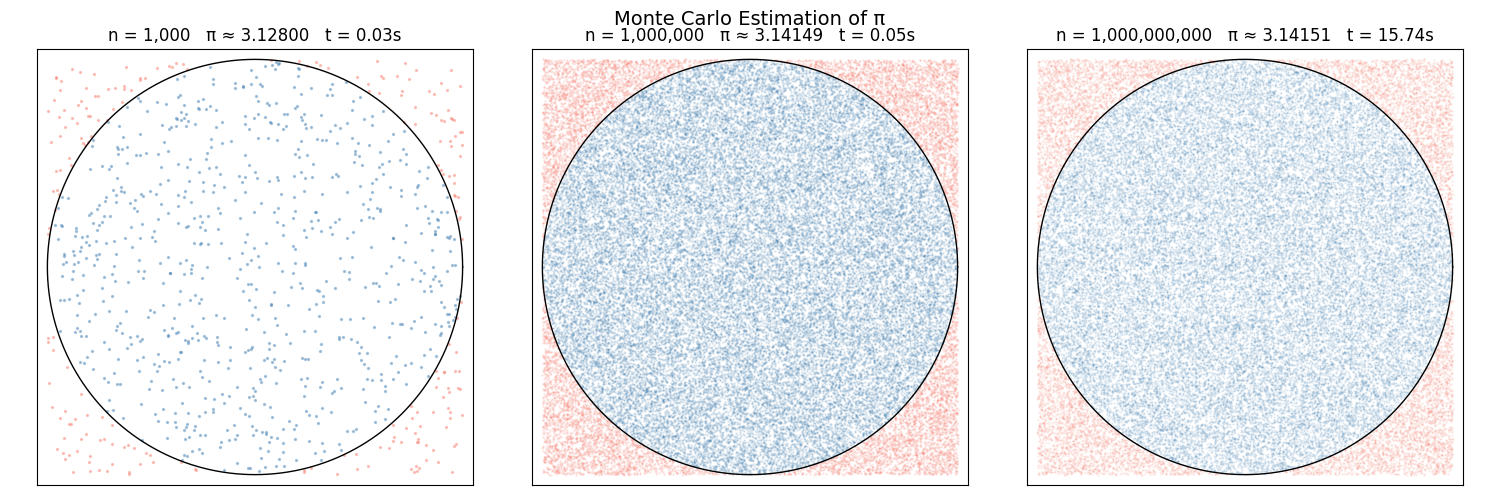
Monte Carlo dart plots at n = 1 000, 1 000 000, and 1 000 000 000. The estimate of π improves with each order of magnitude; the timing shows the cost of that precision.#
Where the Method Is Used#
Monte Carlo techniques appear across computing and science:
Finance — option pricing, Value at Risk
Physics — particle transport, nuclear reactions
Climate modelling — uncertainty quantification
Computer graphics — path tracing for photorealistic rendering
Machine learning — Bayesian inference, dropout regularisation
The idea is always the same: replace an exact but intractable computation with a large number of cheap random samples.
Challenges#
Run
convergence_table([100, 1_000, 10_000, 100_000])several times. Does the error decrease monotonically on every run? Explain why or why not.Add a
seedparameter togenerate_dartsand pass it torandom.seedbefore the loop. Verify that two calls with the same seed produce identical results.The unit circle has area π. Use the same technique to estimate the area of a diamond with vertices at (±1, 0) and (0, ±1). What should the answer be?
Generate two sets of darts with different seeds and save each to its own CSV file. Load both files with
load_darts, concatenate the DataFrames withpd.concat, and computeestimate_pion the combined dataset. Does combining datasets improve the estimate?Plot how the absolute error changes as n increases from 100 to 1 000 000 (use a logarithmic x-axis). Does the slope of the error curve match the expected −½ on a log-log scale?